Soft Sensor Design and Validation for Inferential Quality Control

A soft sensor is a computer program that infers a quality variable, like product concentration or conversion rate, from measurements a plant already collects. The name is a straight mashup of "software" and "sensor": it produces the same kind of real-time reading a physical instrument would, except it never touches the process stream. That distinction matters because the variables plant operators actually care about, the ones that decide whether a batch ships or gets reworked, are often the hardest ones to measure directly.

Consider why. A composition analyzer might cost more than the reactor it's attached to. A flotation cell runs a froth so opaque and chemically hostile that no probe survives contact with it for long. Some measurements are technologically out of reach at any price, given current sensor hardware. The fallback is the lab: pull a sample, run it through gas chromatography or titration, wait twenty minutes to four hours for a result. That delay is the whole problem. By the time the lab number comes back, the process has already moved on, and control decisions made on stale data are, at best, decisions made blind.

Soft sensors close that gap. They take auxiliary variables already sitting in the historian, temperatures, pressures, flow rates, and turn them into a continuous estimate of the variable you actually wanted. But their job doesn't stop at estimation. When a physical analyzer starts to drift from age or a fouled probe, a soft sensor running in parallel gives you something to check it against. That's not a substitute function so much as a diagnostic one in its own right.

What drives the choice between three modeling families

Every soft sensor in production today comes from one of three lineages, and each demands a different relationship with data and process knowledge.

First-principles models sit at one end. Built from mass balances, thermodynamics, reaction kinetics, they can be extremely accurate wherever the underlying chemistry and physics are well understood and well characterized. That's also their limit: complex multiphase systems like froth flotation resist clean mathematical description, and a first-principles model built on shaky assumptions is worse than no model. Where a rigorous model does exist, though, it earns its keep twice over. It works as a sensor in its own right, and it becomes the reference standard against which a data-driven design gets checked, a point that matters for the validation discussion later on.

Data-driven models form the second family, and Partial Least Squares, or PLS, has long been the field's workhorse, a status reflected in its prominent place in the standard soft sensor literature. PLS handles multicollinearity, the condition where predictor variables move together, without falling apart the way ordinary regression does. It stays interpretable, and it's light enough to run on a plant historian server with no dedicated IoT stack behind it. That combination, not raw predictive power, explains why it still appears in new deployments today.

Sparse learners push further on accuracy. RVM and Lasso beat plain PLS in offline testing once you include a lot of time-lagged predictors, cutting minimum prediction error by something in the range of 5 to 10 percent in online settings. RVM comes with a catch, though: its predictions can turn unstable in ways that don't show up until you test them online, so it needs more scrutiny before anyone trusts it with a live loop.

Deep learning covers the nonlinear, dynamic end of the spectrum. CNNs, RNNs, LSTM and bidirectional LSTM networks, and transformers now handle problems that defeated earlier linear methods. Transformer networks have been applied to predict pass/fail outcomes from etching time-series data on semiconductor lines, applications where the failure signature is buried in a long, noisy sequence rather than a single reading. But there's a gap in how these models get built: plenty of published work drops an LSTM into a pipeline without ever checking whether its internal gating mechanism is actually earning its complexity for that dataset. That's an open design question, and it shows in how often these models turn out to be harder to maintain than the accuracy gain justifies. It's an open one, and it shows in how often these models turn out to be harder to maintain than the accuracy gain justifies.

Hybrid approaches are the newest branch, and they try to keep the physics without giving up the fit. Physics-Informed Neural Networks, PINNs, bake conservation laws into the training objective as a regularizer rather than a hard constraint. Physics-guided graph learning goes further, wiring mass-balance relationships directly into a graph neural network's architecture, an approach detailed in a 2024 IEEE Internet of Things Journal paper on physics-enhanced graph neural networks for industrial soft sensing. A 2025 paper on a conditional autoencoder built around a different network structure takes a different angle entirely, aiming for a symbolic, self-interpretable model rather than a black box with a physics patch on top. Even so, hybrid methods run into the same wall first-principles models hit alone: for most industrial processes, nobody has a clean set of differential equations to embed to begin with. Purely data-driven objectives still carry the load in practice, however appealing the hybrid literature looks on paper.

Input selection as the first and most consequential design decision

Before any of those three families gets applied, someone has to decide which measured variables actually go into the model, and that choice affects the model's accuracy and reliability more than which algorithm follows it.

Industrial processes typically carry far more measured variables than any model needs, and throwing all of them in doesn't help. It inflates the variance of parameter estimates, a problem documented at length in the PLS literature: more predictors, especially correlated ones, make the model less certain about each one's contribution, not more accurate overall.

Two mistakes occur repeatedly in how variables get chosen. The first is ignoring time delay. Cause and effect in a process plant never happen at the same instant; a valve move upstream appears downstream ten minutes later, but most causal feature selection methods only look for relationships within a single time slice. That mismatch is baked into the method, not fixed by adjusting a threshold. The second mistake is subtler: standard causal inference techniques assume the candidate variables are decorrelated from each other, and industrial process variables almost never are. Temperature and pressure and flow move together because they're all responses to the same upstream disturbance. Applying a method built on the decorrelation assumption to variables that violate it causes the selection to break down before the modeling even starts.

More advanced feature selection approaches aim to address both problems at once, handling interdependent variables and lagged causal relationships together, rather than treating them as separate issues to patch one at a time. The payoff appears in the numbers: subset selection methods applied to existing refinery sensors can improve accuracy by around 15 percent, a gain that comes entirely from picking better inputs, before any change to the model itself.

Validation before deployment: what rigorous testing requires

A train-test split on historical data is where validation starts, not where it ends. Every soft sensor should clear that bar, but clearing it only proves the model fits data it's already seen shuffled into two piles. It says nothing about how the model handles a process condition it has never encountered.

Where a rigorous first-principles model exists for the process, it gives you an independent check that historical data alone can't. Cases discussed in the inferential sensor literature show the pattern: a data-driven soft sensor's outputs are checked against an independent reference to confirm that the sensor is accurate enough to feed an advanced process control scheme.

In most plants, though, the real ground truth is intermittent lab data, samples pulled every few hours and run through an analyzer or a wet-chemistry method. Validation protocols need to be built around that cadence, around the actual lab sampling schedule, not around whatever fit statistic the modeling software reports by default. A soft sensor that scores well on R² against training data but drifts steadily between lab samples will fail in exactly the way that matters to an operator, quietly and for hours at a stretch.

None of this is a one-time checkbox, either. Treating a soft sensor as a classical machine learning model with a single held-out test set misses what deployment actually demands: continuous monitoring once it's live, defined triggers for when to retrain it, and a record of exactly which data version trained which model. That's the MLOps discipline applied to a soft sensor, and skipping it is how models degrade without anyone noticing until the deviation is large enough to cost money.

Online monitoring: detecting when a deployed soft sensor is no longer trustworthy

The dangerous failure mode for a soft sensor isn't a crash. The dangerous failure mode for a soft sensor isn't a crash but silence. The process drifts, the true quality variable moves away from where the model thinks it is, and the sensor keeps reporting a confident number built on an assumption that stopped being true. No alarm fires, because nothing has technically broken.

One layer of defense checks the inputs themselves. If a temperature or flow measurement feeding the soft sensor goes faulty, any target value the model hands to an MPC controller downstream is now built on bad information, whether or not the soft sensor's own math is still correct. Detecting a faulty input sensor and reconstructing a reasonable value for it in real time is what keeps the control loop running through a hardware failure, instead of forcing a shutdown every time an instrument fails.

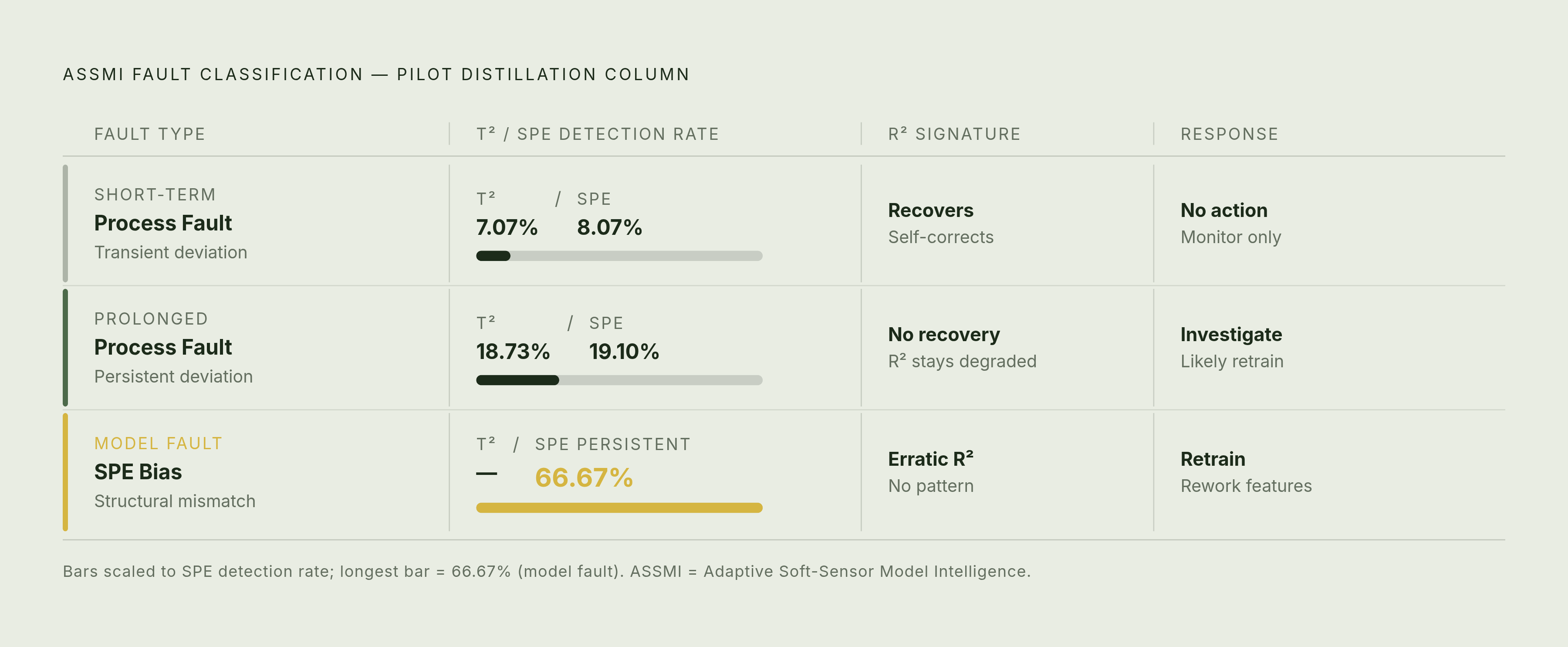
A framework called Automated Statistical Soft Sensor Monitoring and Intervention, or ASSMI, tested this logic against a pilot-scale distillation column in Aspen Dynamic Simulation, running three separate fault scenarios, with results published in Results in Engineering in 2025. The findings split cleanly by fault type. Short-term faults triggered low detection rates, 7.07 percent on the T² statistic and 8.07 percent on SPE, and the model's R² recovered quickly on its own. The interpretation: these are self-correcting blips, and stepping in with a retrain would waste effort and risk destabilizing a sensor that was already fixing itself. Prolonged process faults told a different story, higher detection rates at 18.73 percent and 19.10 percent, with no R² recovery at all, so the fault needs actual investigation and the model likely needs updating. Model faults were the clearest case: 66.67 percent persistent bias on SPE with erratic R² behavior, a signature that points straight at retraining or reworking which features feed the model.

Not every deviation deserves the same response, and that principle underneath ASSMI carries forward. Telling the fault types apart lets a plant respond to what's actually wrong instead of retraining reflexively every time a number moves, which saves maintenance effort and avoids the real risk of destabilizing a sensor that would have corrected itself given a few more cycles.

Bias update and adaptive correction for ongoing model accuracy

Bias update is a smaller, more frequent intervention than retraining, and it does a different job. Rather than touching the model's underlying structure, it nudges the sensor's output during normal operation to correct for the small inaccuracies that build up as conditions shift, without ever tearing the model down and rebuilding it.

The mechanism has a safeguard built in. Feedback error, the gap between the soft sensor's estimate and a lab result or reference measurement, doesn't get applied to the model raw. It goes through a statistical significance check first, and the correction only fires when that error is large enough to be a real signal rather than noise. That single filtering step is what keeps a bias update scheme from overcorrecting on every minor fluctuation in the lab number, which would just add a new source of instability.

There's a second use for that bias signal beyond correction, too. When it stays persistently large instead of settling back down, that's not just something to patch. It's a sign that the process itself has shifted, or that an input sensor somewhere has drifted out of calibration, and it should be investigated on those terms rather than folded into the correction and moving on. Bias update of this kind isn't a research curiosity: it appears as a practical maintenance mechanism across the applied soft sensor literature, which says something about how essential the plant floor considers it.

Handling concept drift and cross-condition adaptation through transfer learning

Every soft sensor built offline starts decaying the moment it goes live, in a slow and well-documented way. Raw material batches change supplier. Catalyst deactivates over months of runtime. Fouling builds up on a heat exchanger surface. Seasonal shifts change cooling water temperature. None of these appears as a single dramatic fault, but together they constitute concept drift, and it is one of the most consistently reported problems in the applied soft sensor literature.

Recent work reframes drift less as a decay problem and more as a domain adaptation problem, treating the sensor's original training conditions as one domain and its current operating conditions as another. Optimal transport transfer learning is one solution proposed on those terms. Gaussian mixture domain adaptation and deep subdomain learning adaptation networks are others, each trying to map what the model learned under old conditions onto what's true under new ones, without starting from zero.

The broader transfer learning literature sorts these approaches into four categories: instance-based, feature-based, parameter-based, and relational knowledge transfer. A graph-based predictable deep transfer network is a concrete example of the last category, using the physical topology of the process itself, which unit feeds which, how streams connect, as structural information the model can lean on when adapting to a new operating regime. That's a meaningfully different strategy from just feeding a model more data and hoping it generalizes; it gives the adaptation a map to follow.

Deployment across sectors and the industrial record

Refining and petrochemicals represent one of the most extensively documented industries for soft sensor deployment, and the record is a plain one: these systems have been running continuously for years, not months, in the plants that adopted them early.

A chemical company in Japan deployed LW-PLS soft sensors and inferential control on a cracked gasoline fractionator and on the purification section of an acetyl plant. Both systems ran for more than a year in production. The cracked gasoline fractionator alone cut operating cost by around 0.6 percent, a figure that reads as modest until you remember what 0.6 percent means at refinery throughput: a small percentage translating into a large absolute number, sustained across every day the system stayed online.

Fermentation and bioprocessing present a different set of demands, and a 2025 paper by Metcalfe and colleagues in Computers & Chemical Engineering, describing a soft sensor built on an operational machine-learning pipeline for real-time prediction in industrial-scale fed-batch fermentation, lays out why. Batches vary from run to run in ways a continuous chemical process doesn't. Labeled data is scarce, because every label requires a lab assay on a live culture. And there's rarely an inline analyzer capable of tracking product quality in real time at all, which makes the soft sensor not a nice-to-have alternative to hardware measurement, but the only real-time option on the table.